Category Archives: Machine Learning

Iterative Dichotomiser 3 (ID3) algorithm – Decision Trees – Machine Learning

ID3 is the first of a series of algorithms created by Ross Quinlan to generate decision trees.


Characteristics:

  • ID3 does not guarantee an optimal solution; it can get stuck in local optimums
  • It uses a greedy approach by selecting the best attribute to split the dataset on each iteration (one improvement that can be made on the algorithm can be to use backtracking during the search for the optimal decision tree)
  • ID3 can overfit to the training data (to avoid overfitting, smaller decision trees should be preferred over larger ones)
  • This algorithm usually produces small trees, but it does not always produce the smallest possible tree
  • ID3 is harder to use on continuous data (if the values of any given attribute is continuous, then there are many more places to split the data on this attribute, and searching for the best value to split by can be time consuming).


Alternatives:

  • ID3 is a precursor to both C4.5 algorithm, as well as C5.0 algorithm.
  • C4.5 improvements over ID3:
    • discrete and continuous attributes,
    • missing attribute values,
    • attributes with differing costs,
    • pruning trees (replacing irrelevant branches with leaf nodes)
  • C5.0 improvements over C4.5:
    • several orders of magnitude faster,
    • memory efficiency,
    • smaller decision trees,
    • boosting (more accuracy),
    • ability to weight different attributes,
    • winnowing (reducing noise)
  • J48 is an open source Java implementation of the C4.5 algorithm in the Weka data mining tool
  • C5.0 is being sold commercially (single-threaded version is distributed under the terms of the GNU General Public License) under following names: C5.0 (Unix/Linux), See5 (Windows)


Usage:

  • The ID3 algorithm is used by training a dataset S to produce a decision tree which is stored in memory.
  • At runtime, the decision tree is used to classify new unseen test cases by working down the tree nodes using the values of a given test case to arrive at a terminal node that tells you what class this test case belongs to.


Metrics:

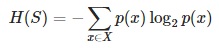
  • Entropy H(S) – measures the amount of uncertainty in the (data) set S
  • Information gain IG(A) – measures how much uncertainty in S was reduced, after splitting the (data) set S on a attribute
  • More details on both Entropy and Information Gain you’ll find here.


High-level inner workings:

  • Calculate the entropy of every attribute using the data set S
  • Split the set S into subsets using the attribute for which entropy is minimum (or, equivalently, information gain is maximum)
  • Make a decision tree node containing that attribute
  • Recurse on subsets using remaining attributes


Detailed algorithm steps:

  1. We begin with the original data set S as the root node
  2. In each iteration the algorithm iterates through every unused attribute of the data set S and calculates the entropy H(S) (or information gain IG(A)) of that attribute
  3. Next it selects the attribute which has the smallest entropy (or largest information gain) value
  4. The data set S is then split by the selected attribute (e.g. age < 50, 50 <= age < 100, age >= 100) to produce subsets of the data
  5. The algorithm continues to recurse on each subset, considering only attributes never selected before
  6. Recursion on a subset may stop in one of these cases:
    • every element in the subset belongs to the same class (+ or -), then the node is turned into a leaf and labelled with the class of the examples
    • there are no more attributes to be selected, but the examples still do not belong to the same class (some are + and some are -), then the node is turned into a leaf and labelled with the most common class of the examples in the subset
    • there are no examples in the subset, this happens when no example in the parent set was found to be matching a specific value of the selected attribute, for example if there was no example with age >= 100. Then a leaf is created, and labelled with the most common class of the examples in the parent set
  7. Throughout the algorithm, the decision tree is constructed with each non-terminal node representing the selected attribute on which the data was split, and terminal nodes representing the class label of the final subset of this branch


Python implementation:

  1. Create a new python file called id3_example.py
  2. Import logarithmic capabilities from math lib as well as the operator library
        from math import log
        import operator
    
  3. Add a function to calculate the entropy of a data set
    def entropy(data):
        entries = len(data)
        labels = {}
        for feat in data:
            label = feat[-1]
            if label not in labels.keys():
            labels[label] = 0
            labels[label] += 1
        entropy = 0.0
        for key in labels:
            probability = float(labels[key])/entries
            entropy -= probability * log(probability,2)
        return entropy
    
  4. Add a function to split the data set on a given feature
    def split(data, axis, val):
        newData = []
        for feat in data:
            if feat[axis] == val:
                reducedFeat = feat[:axis]
                reducedFeat.extend(feat[axis+1:])
                newData.append(reducedFeat)
        return newData
    
  5. Add a function to choose the best feature to split on
    def choose(data):
        features = len(data[0]) - 1
        baseEntropy = entropy(data)
        bestInfoGain = 0.0;
        bestFeat = -1
        for i in range(features):
            featList = [ex[i] for ex in data]
            uniqueVals = set(featList)
            newEntropy = 0.0
            for value in uniqueVals:
                newData = split(data, i, value)
                probability = len(newData)/float(len(data))
                newEntropy += probability * entropy(newData)
            infoGain = baseEntropy - newEntropy
            if (infoGain > bestInfoGain):
                bestInfoGain = infoGain
                bestFeat = i
        return bestFeat
    
  6. According to step 6 of the “Detailed algorithm steps” section above, there are certain cases in which the recursion may stop. If we don’t meet any of the stopping conditions, then the small function below will allow us to choose the best feature depending on the “majority”:
    def majority(classList):
        classCount={}
        for vote in classList:
            if vote not in classCount.keys(): classCount[vote] = 0
            classCount[vote] += 1
        sortedClassCount = sorted(classCount.iteritems(), key=operator.itemgetter(1), reverse=True)
        return sortedClassCount[0][0]
    
  7. Finally add the main function to generate the decision tree
    def tree(data,labels):
        classList = [ex[-1] for ex in data]
        if classList.count(classList[0]) == len(classList):
            return classList[0]
        if len(data[0]) == 1:
            return majority(classList)
        bestFeat = choose(data)
        bestFeatLabel = labels[bestFeat]
        theTree = {bestFeatLabel:{}}
        del(labels[bestFeat])
        featValues = [ex[bestFeat] for ex in data]
        uniqueVals = set(featValues)
        for value in uniqueVals:
            subLabels = labels[:]
            theTree[bestFeatLabel][value] = tree(split\(data, bestFeat, value),subLabels)
        return theTree


Voilà


Resources:


Measuring Entropy (data disorder) and Information Gain

This is a very short post about two of the most basic metrics in the Information Theory


Entropy:

  • is a measure of the amount of uncertainty in the (data) set S (i.e. entropy characterizes the (data) set S).
  • in other words, it is the average amount of information contained in each message received (message here stands for an event, sample or character drawn from a distribution or data stream)
  • it characterizes the uncertainty about our source of information (Entropy is best understood as a measure of uncertainty rather than certainty, as entropy is larger for more random sources)
  • a data source is also characterized by the probability distribution of the samples drawn from it (the less likely an event is, the more information it provides when it occurs)
  • it makes sense to define information as the negative of the logarithm of the probability distribution (the probability distribution of the events, coupled with the information amount of every event, forms a random variable whose average (expected) value is the average amount of information (entropy) generated by this distribution).
  • because entropy is average information, it is also measured in shannons, nats, or hartleys, depending on the base of the logarithm used to define it


Math interpretation:

Entropy_1


Entropy_2


Entropy_3


Python implementation:

# Calculates the entropy of the given data set for the target attribute.
def entropy(data, target_attr):

    val_freq = {}
    data_entropy = 0.0

    # Calculate the frequency of each of the values in the target attr
    for record in data:
        if (val_freq.has_key(record[target_attr])):
            val_freq[record[target_attr]] += 1.0
        else:
            val_freq[record[target_attr]]  = 1.0

    # Calculate the entropy of the data for the target attribute
    for freq in val_freq.values():
        data_entropy += (-freq/len(data)) * math.log(freq/len(data), 2) 

    return data_entropy


Information Gain:

  • is the measure of the difference in entropy from before to after the data set S is split on an attribute A
  • in other words, how much uncertainty in S was reduced after splitting data set S on attribute A
  • it is a synonym for Kullback–Leibler divergence (in the context of decision trees, the term is sometimes used synonymously with mutual information, which is the expectation value of the Kullback–Leibler divergence of a conditional probability distribution. The expected value of the information gain is the mutual information I(X; A) of X and A – i.e. the reduction in the entropy of X achieved by learning the state of the random variable A. In machine learning, this concept is used to define a preferred sequence of attributes to investigate to most rapidly narrow down the state of X. Such a sequence (which depends on the outcome of the investigation of previous attributes at each stage) is called a decision tree. Usually an attribute with high mutual information should be preferred to other attributes).


Math interpretation:

Information_Gain_1


Information_Gain_2


Python implementation:

# Calculates the information gain (reduction in entropy) that would result by splitting the data on the chosen attribute (attr).
def gain(data, attr, target_attr):

    val_freq = {}
    subset_entropy = 0.0

    # Calculate the frequency of each of the values in the target attribute
    for record in data:
        if (val_freq.has_key(record[attr])):
            val_freq[record[attr]] += 1.0
        else:
            val_freq[record[attr]]  = 1.0

    # Calculate the sum of the entropy for each subset of records weighted by their probability of occuring in the training set.
    for val in val_freq.keys():
        val_prob = val_freq[val] / sum(val_freq.values())
        data_subset = [record for record in data if record[attr] == val]
        subset_entropy += val_prob * entropy(data_subset, target_attr)

    # Subtract the entropy of the chosen attribute from the entropy of the whole data set with respect to the target attribute (and return it)
    return (entropy(data, target_attr) - subset_entropy)


Cheers!


Resources:

k-Nearest Neighbors (kNN) algorithm – Machine Learning

k-Nearest Neighbors (kNN) is an easy to grasp algorithm (and quite effective one), which:

  • finds a group of k objects in the training set that are closest to the test object, and
  • bases the assignment of a label on the predominance of a particular class in this neighborhood.


There are three key elements of this approach:

  • a set of labeled objects, e.g., a set of stored records (data),
  • a distance or similarity metric to compute distance between objects,
  • and the value of k, the number of nearest neighbors.


To classify an unlabeled object/item:

  • the distance of this object to the labeled objects is computed,
  • its k-nearest neighbors are identified,
  • and the class labels of these nearest neighbors are then used to determine the class label of the object.


Figure below provides a high-level summary of the nearest-neighbor classification algorithm.


knn_example1


knn_example2


Distances are calculated using the Euclidian distance, where the distance between two vectors, xA and xB, with two elements, is given by:

knn_example_euclidian


k-Nearest Neighbors Pros vs. Cons:

  • Pros – High accuracy, insensitive to outliers, no assumptions about data
  • Cons – Computationally expensive, requires a lot of memory
  • Works with – Numeric values, nominal values


Prior to starting coding, here’s what we assume we have: (details in Peter Harrington’s exceptional “Machine Learning in Action”)

  • We have the training data (an existing set of example data)
  • We have labels for all of this data
  • We know what class each piece of the data should fall into
  • When we’re given a new piece of data without a label, we compare that new piece of data to the existing data (every piece of existing data)
  • We then take the most similar pieces of data (the nearest neighbors) and look at their labels
  • We look at the top k most similar pieces of data from our known dataset; this is where the k comes from
  • Lastly, we take a majority vote from the k most similar pieces of data, and the majority is the new class we assign to the data we were asked to classify


I’ll be using Python (v3.3.5) programming language for code examples:

  1. Create a text file named “test_data.txt” that will contain our test data set (x,y coordinates/pairs of points in a 2D space together with labels (3rd column))
        0.2    1.3    top-left
        0.1    1.1    top-left
        0.9    0.1    bottom-right
        1.0    0.2    bottom-right
    
  2. Create a new python file called knn_example.py
  3. Import NumPy (package for scientific computing) and the Operator module (sorting tuples). NumPy requires previous installation from here.
        from numpy import *
        import operator
    
  4. Add a function to prepare the data set (load it from the file and transform into data(matrix) and labels(vector) components)
        def prepareData(fname):
            file = open(fname)
            lines = len(file.readlines())
            data = zeros((lines,2))
            labels = []
            file = open(fname)
            i = 0
            for line in file.readlines():
                line = line.strip()
                list = line.split('\t')
                data[i,:] = list[0:2]
                labels.append(list[-1])
                i += 1
            return data,labels
    
  5. Add a function to classify the data
        def classify(x, data, labels, k):
            size = data.shape[0]
            diff = tile(x, (size,1)) - data
            sqDiff = diff**2
            sqDist = sqDiff.sum(axis=1)
            dist = sqDist**0.5
            sortedDist = dist.argsort()
            count={}
            for i in range(k):
                label = labels[sortedDist[i]]
                count[label] = count.get(label,0) + 1
            sCount = sorted(count.items(), key=operator.itemgetter(1), reverse=True)
            return sCount[0][0]
    
  6. Save the file
  7. Execute (from Python CLI or IDLE):
        >>> import knn_example
        >>> group,labels = knn_example.prepareData('test_data.txt')
        >>> knn_example.classify([1,0], group, labels, 2)


What you should see after executing the above, is following:

    'bottom-right'


Voila, you just created your first classifier (which successfully classified a point with x,y coordinates of 1,0 by assigning it the ‘bottom-right’ label)


Resources: